
Over the years I spent a lot of time writing simulation or data processing code for some kind of data. While some data sets are very small (just a few hundred values) it not uncommon today to have a few dozen, a few hundred or even a few thousand megabytes of data to process in some way. In fact, Python is in many cases well capable of processing such data with performance comparable to e.g. C, but with vastly more readable and especially writeable code.
This article writes down some thoughts and findings on how to do this more efficiently with Python code, and focuses specifically on the situation I find myself in most commonly: What counts is the overall amount of time you need to obtain a certain result, i.e. development time plus runtime of the program. I do not want to discuss Python vs C / Fortran / C++ / whatever: it is clear you can always be faster with a compiled language. But if you can get to 40% of the performance of a C program with Python by writing just a hundreth as much code, it’s probably much faster (and much less painful) overall in practice. I will write down a few basics first but mostly focus on a few more hidden features and tricks later on.
So, basics first:
Vectorize everything!
The basis of all scientific data processing in Python today is the numpy module. It provides an array class, numpy.array, which can be used to store numbers, bascially. Whenever you have some numbers, you most probably want to store them in a np.array. You can select a data type (e.g. float32, float64, int), but the default (float64 for most input) is usually fine.
Anyways: Do not loop over np.array instances. In 99% of cases where people do that, it’s the wrong thing to do. Why? Because it is super slow. For a loop, each individual number is converted to a python object; type checks occur, type casts may happen, null checks happen, checks for exceptions in the operator happen, all kinds of things. If you write 3+5 in Python, it will execute hundreds, if not thousands of lines of C code in the background. And that happens for each number in your array if you loop over it. (The same goes for things like a = np.array([x**2 for x in range(50)]), that generator is a loop as well). So, what to do instead?
Operate on the full array without using a loop
For many operations such as adding, dividing etc, this is trivial, just write a+b where a and b are np.array instances. This just adds the Python overhead one single time — for maybe ten million numbers to add in a and b, which makes it completely negligible. The actual iteration happens in a very fast machine-code loop.
All numpy mathematical functions operate on arrays. If you want to calculate the sine of a thousand values, put them into an array and write np.sin(a). Even complicated functions such as np.fft.rfft take an array of input vectors. For some functions, you need to specify the axis they should operate on.
This should also affect how you write your functions and classes: If possible at all, make your functions such that they can operate on a whole array of values, not just a number. And trust me: it is almost always possible, and for most operations it’s as simple as “use np.sqrt instead of math.sqrt”. Do not store your “objects” (e.g. simulated particles) in individual Python objects; instead, use one Python object for the whole collection of simulated particles, and have e.g. the positions and velocities as np.array instances in that object.
This “use the full array” rule is also true if your array has more than one dimension. Often things require a bit more thinking for multi-dimensional arrays, but in almost all cases it’s still possible to avoid a python loop. Avoid python loops at all costs; whatever you do with numpy’s builtin functions will be faster, and probably much faster.
Use numpy’s data reduction functions
If you want to know the sum of all values in an array, use np.sum. If you want to know the absolute value of an array of position vectors, use np.sqrt(np.sum(x**2, axis=1)). Use np.reshape to compute averages: np.average(np.reshape(x, -1, average_count), axis=1). The most useful thing about reshape I learned one day is that you can give -1 for any one dimension to have the function calculate it automatically.
If you want to categorize/bin values of an array, use np.histogram (note also np.histogramdd which computes multi-dimensional histograms).
Use numpy’s data generation functions
numpy can generate random numbers in various distributions, as well as arrays initialized with ones, zeros, or ranges of numbers in all sizes. Make sure to use those functions, instead of initializing an array in a loop. A few functions to look at are np.random.normal, np.random.uniform, np.zeros, np.zeros_like, np.arange and np.linspace. Make sure you know how those work; all of them are worth it.
Although np.arange feels more “at home” for python because it is basically the built-in range(), I find np.linspace to be more useful in many situations, since it allows you to adjust the range while keeping the amount of values. And the amount of values is often more important than their exact positions.
Cleverly use slicing
If you want to know the difference between one element and the next, use slicing: x[1:] – x[:-1]. Make sure you know what np.newaxis is for. Consider using slices with ellipses.
This was just a short overview of a few basic concepts. There are enough introductions to numpy out there, I don’t want to replicate those. The rest of the article is on some more specialized findings.
Use np.einsum
np.einsum is not exactly the simplest function in the world to understand, but it is very powerful and allows efficient vectorization of almost any operation that requires multiplying elements from two arrays and adding them up subsequently. The most obvious use case is matrix multiplication; for example, you can multiply an array of rotation matrices with an array of vectors: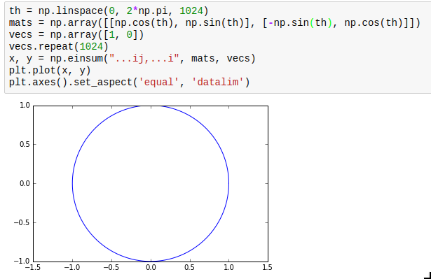
Use np.interp and np.cumsum
This is not so much about performance but instead usability. The interp (“interpolate”) and cumsum (“cumulative sum”) functions actually quite often are what you want but sometimes it’s hard to realize this. Especially, you can use them for numeric integration and inverting functions. interp is of course also very useful in its most obvious application, which is re-sampling data to a grid.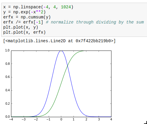
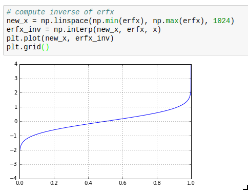 This makes it for example very simple to calculate inverse cumulative distribution functions as required for drawing weighted random numbers.
And remember, all this has basically the same performance like C code. Try doing that in C. For example, compare this numpy-vectorized implementation of 4th order Runge Kutta to the C one on wikibooks: comparably fast, and vastly more readable.
Sacrifice your soul, errr, memory for performance
Sometimes you can only vectorize things when you sacrifice a bit of memory. A typical case is a system of interacting particles. The interaction will usually depend on the distance between the two particles; so for an array x of 3d coordinates, you need the distance between each pair of particles. One way to write this down without using a python loop is as follows: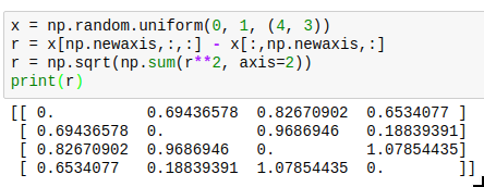
The resulting entries r[i][j] will contain the distance between particle i and j. The downside is that you need to allocate twice as much memory as you would actually need to store all the distances, and also need twice the computation time because the result is symmetric but you cannot use that knowledge. Neverthereless, this is vastly faster than the python loop version, and allows you to use the r array in a vectorized version of your energy (or force) function.
Use masks
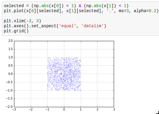
Another thing which is easy to miss is the use of masks. The idea of masks is that you can index an array with an array of compatible size containing just True and False (such arrays have data type np.bool). The elements where the corresponding slice array entry is True are selected; the others are not. The result of such a mask access is writeable. Additionally, using operators such as > or < on arrays gives you such a mask.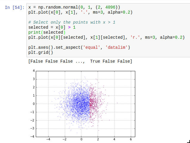 The next thing you need to know about masks is that the bitwise operators | and & work on them to take the union or intersect of two masks. A third one which is useful is ~ which inverts a mask.
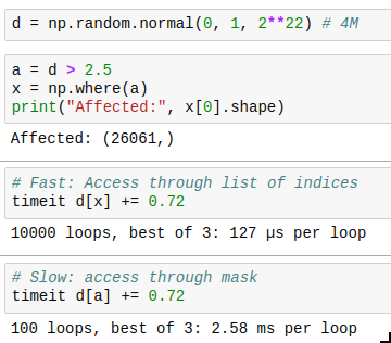
 And there is one last thing to know: you can get the indices where a mask is True by using np.where(). The performance trick here is that if you only want to operate on a few indices, you can first find those by combining a few masks, then get the indices by using np.where, and then only acces those indices, which is much faster than by using the full mask every time. Compare for yourself:
You can count the amount of entries in your mask with np.ma.count(), or find out if any or all entries are masked with .any() and .all().
Avoid copying arrays in critical sections
In general, copying data is cheap. But if your program simulates 25 million particles, each having a float64 location in 3d, you already have 8*3*25e6 = 600 MB of data. Thus, if you write r = r + v*dt, you will copy 1.2 GB of data around in memory: once 600 MB to calculate v*dt, and again to calculate r+(v*dt), and only then the result is written back to r. This can really become a major bottleneck if you aren’t careful. Fortunately, it is usually easy to circumvent; instead of writing r = r+dv, write r += dv. Instead of a = 3*a + b, write a *= 3; a+= b. This avoids the copying completely. For calculating v*dt and adding it to r, the situation is a bit more tricky; one good idea is to just have the unit of v be such that you don’t need to multiply by dt. If that is not possible, it might even be worth it to keep a copy of v which is multiplied by dt already, and update that whenever you update v. This is advantageous if only few v values change per step of your simulation.
I would not recommend writing it like this everywhere though, it’s often not worth the loss in readability; just for really large arrays and when the code is executed frequently.
Note that this consideration does not apply to indexing usually, as indexing does not copy an array but just creates a view of it.
And, as always, be sure to profile your application: python -m cProfile -s tottime yourscript.py. It’s very often surprising what shows up, and the ten minutes you spend running the profiler and fixing the top three pointless bottlenecks will pay off in simulation time in less than a day, I guarantee it.
Use binary data files
Numpy provides very easy, very fast ways to read and write arrays from files. To load some CSV, use np.loadtxt. However, as soon as you have more than a few MB of CSV, this starts to get kind of slow. I really recommend to use np.load and np.save instead, which load from and save to a binary format. This is so much faster that it is frequently a good step to convert data which initially is presented in a CSV to you to a binary file (just load it with np.loadtxt and save it again with np.save) before doing anything else.
There are also versions with compression if you need that.
np.load and np.save are also a very good way to cache intermediate results of your computation. If there’s something your program does every time, just add a command line flag to actually do it and write it to a cache file, and if that flag is not given load it from there instead. It’s two lines of code, and if what you do takes more than second, it’s really worth it in the long run.
Misc
numpy includes some utility methods for floating point handling. If you want to test that something is normalized to 1, you can e.g. use np.allclose(x, 1). Note that you shouldn’t use (x == 1).all(), floating point and exact comparison doesn’t mix well. Those methods also include checking for nan values which is sometimes useful, especially you can do x[np.isfinite(x)] to only get the valid values out of x (i.e. not nan or inf).
I hope you found a new thing or two while reading this article 🙂
P.S.: The right way to import numpy is to write “import numpy as np” or “import numpy”. Not “from numpy import *”. The latter clutters your namespace, and makes it very hard to know which function(s) are actually from numpy and which ones are not.
Categories: Everything
Tags: numpy, performance, planetkde, python
8 replies ›
Trackbacks
- Brauch: Processing scientific data in Python and numpy, but doing it fast | Linux Press
- Brauch: Processing scientific data in Python and numpy, but doing it fast | Dentoron Linux App
- Links 18/4/2016: Linux 4.6 RC4, Tomb Raider for GNU/Linux | Techrights
If dealing with tabular data, use pandas (https://pandas.pydata.org). It makes things easier.
And dates too, I think. Last time I checked numpy’s datetime handling was still kind of terrible.
I work at the Spanish Weather service in Catalonia and my colleagues and I also use Pandas often for data processing. It is actually built upon Numpy and makes things somewhat easier.
Thanks for the article. I learned many of these things from
experience, so having them compiled in an article is great!
Very interesting, I’ve been wondering about numpy for awhile and the tips are excellent. Do you have any particle demos to show?
Unfortunately not right now, I only have some things which are fairly boring and some things which are fairly interesting but which I cannot publish 😉